Aircraft and Radar Observations of Supercooled Liquid Water
Damian Wilson
A frontal system passed over southern England on March 30th 1999 and was
observed by both the Chilbolton radar in Hampshire and the Met. Research
Flight C130. The comparison of the aircraft and radar data has been written up
by Robin Hogan at the University of Reading and is presented
here. This note
summarizes how the model performed in relation to these observations.
The main point to note from the observations is that liquid water is confined
to upward moving plumes of moisture, which have not had time to produce ice.
Quantitative values were measured by the aircraft. These regions are associated
with to high values of differential reflectivity (ZDR) within a frontal
system. These
features are relatively common in frontal systems, and therefore radar has
the potential to pick out (and perhaps measure?) regions of supercooled water.
As I will present below, the model gives a similar impression, but there
are significant differences.
To ensure a reasonable spinup of the model I will present a T+6 mesoscale
forecast from the 6Z analysis (so verifying at 12Z 30/3/99). I will look at
cross sections from Chilbolton to a range of 80km at an azimuth of 250 degrees.
These are similar to those presented by Robin.
The results from a control run using the
3B mixed phase scheme are shown here:
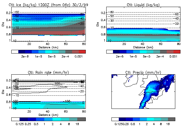
The dotted lines in each cross section are
the temperature (in degrees C), and the solid lines in the bottom left panel
the relative humidity (in percent, with respect to ice). The air is saturated
from the melting layer to about 250hPa, with slight supersturation in places.
The eta levels correspond roughly to the heights: (1.0 - surface; 0.8 - 1750 m
; 0.6 - 4100 m; 0.4 - 7000 m; 0.2 11500 m). There are approximately seven grid
points across the domain shown.
- Ice content: This shows little variation across the domain, in
contrast to that inferred by the radar from the reflectivity (Z). There is
a substantial amount of ice at the melting layer, and a slight increase
at longer range.
- Liquid content: This is confined to temperatures warmer than -10
deg C and rapidly increases towards the melting layer. There is a uniform, thin
layer of high liquid content at the melting layer. Note that the liquid
tends to decrease with range, in contrast to the ice. This is due to greater
deposition and riming rates at the longer ranges. Comparison of the liquid
contents to those measured by the aircraft produces reasonable agreement.
- Rainfall rate: Not surprisingly, this increases at the larger
ranges. Note also, that the rainrate is very heavy. The model is probably
over estimating the rate. A T+0.5 run from the 12Z analysis produced much
less rain, but may not be properly spun up.
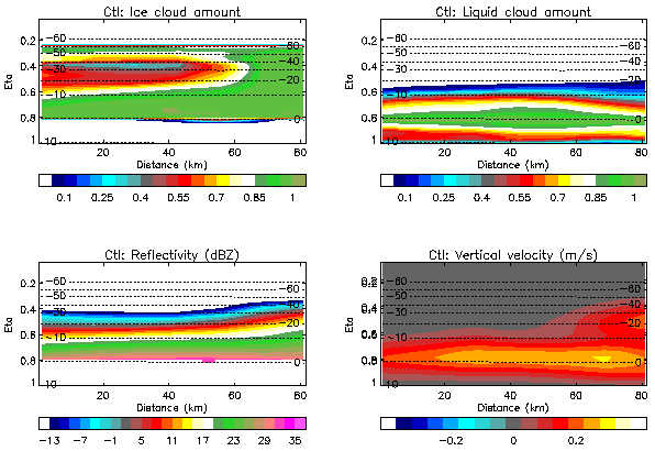
- Ice cloud amount: This shows almost solid cloud at altitudes below
4000m,
but also broken cloud at higher altitudes at the shorter ranges. The radar
images show solid cloud to higher levels than this. The underestimate of cloud
at these altitudes by the scheme is already known and the cloud fraction scheme
is being revised.
- Liquid cloud amount: This is more difficult to verify, but the
aircraft data shows only occasional plumes of liquid, which probably have a
fractional coverage which does not decrease with height as dramatically as
the model predicts. The large liquid cloud amounts predicted by the model
towards the melting layer are also likely to be overestimated. Since the water
contents appear to be reasonable, this suggests that the distribution function
of the moisture in the gridbox does not have an extreme enough tail (at
high contents). This is consistent with a model of a few, rapidly ascending
plumes.
- Radar reflectivity: This can be directly compared with the
observations. This suggests that reflectivities are predicted to be too high
(the same is true of the rainfall reflectivities). This will be mainly due
to the over development of the system in the model (or an error in its
positioning). The radar echo top is reasonably well predicted, as is the
general rise in top at longer range. The radar shows large changes in
reflectivity on scales below that of a gridbox (12km) whereas the model
shows changes only on scales much larger than this.
- Vertical velocity (of air): The upward motion of the air is very
significant,
especially at lower levels. Note that the range of largest ice content
corresponds to the range of the largest vertical velocities - more moisture is
transported to higher levels. However, on a small scale (shown by the radar)
the ice content is reduced in updraughts - the ice has not had time to grow.
The modelled vertical motion is likely to be too large in this simulation.
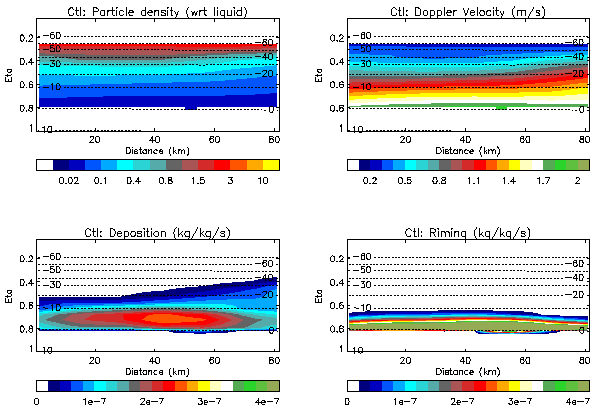
- Particle density: The model predicts a decrease in mean density
from the upper layers to around 0.05 closer to the melting layer, which is
qualitatively reasonable at least.
- Doppler velocity: The vertical air velocity should be subtracted
from this to obtain the downwards Doppler velocity that would be measured
from a vertically pointed radar (for Rayleigh scattering). The particles fall
faster as they get larger. Since the radar was scanning rather than pointing
vertically a comparison with observations is difficult.
- Deposition and riming rates: These have been included to show that
the main conversion of mass to ice comes from depositional growth rather than
riming. However, riming becomes very significant just above the melting layer.
It is possible that aircraft observations of ice particle shapes may be able
to (qualitatively) validate this prediction.
Some conclusions follow on from the above discussion. Points marked by *'s
might be possible to validate from aircraft or radar. Points marked highlighted
in red are those which I think are the most important
for development work.
- The exact positioning of the system in the model is very important
- There is little variation in the model over a scale of 80km, and certainly
no structure resolved on the grid-scale.
- There is a modelled band of liquid at the melting layer.*
- The modelled liquid content reduces as cloud top rises.* This is opposite
to the change observed over short distances near the updraughts. Is the
behaviour over longer distances more reminisecent of the model?
- Note that modelling work from UMIST suggests that
periodic ascending
plumes of moisture increases the mean ice content but the mean liquid content
remains unchanged (relative to a uniform cloud base vapour flux). *?
- The subgrid variation of vapour and liquid in the model
is not as great as
it should be (at the moist end of the distribution). This is the opposite
conclusion to that drawn from studies of warm stratocumulus clouds.
- Lidar measured cloud base is very low, consistent with the model
predictions. No bases higher than the melting layer were observed, although
nearly always the lowest cloud was observed lower than this.
- Cloud top defined by reflectivity is reasonably predicted by the model.
- Although a little high, the modelled radar reflectivity is reasonable.
This will depend largely on the successful prediction of the dynamics.
- Riming is very intense near the melting layer whereas deposition peaks
higher up in the cloud.*
- Average modelled particle densities decrease from 0.8 at modelled cloud
top to around 0.02 at the melting layer.*
- Doppler velocities due to falling ice are around 1 - 1.5 m/s.
- Modelled cloud fraction is too low towards the radar
cloud top (at mid levels).
- The ice content has not been validated from this work
(although
reflectivity has). *
Although individual case studies yield valuable information there is a need
to remove some of the variable nature of such comparisons caused by the model
not predicting the correct dynamical behaviour of the system. This could
be looked at by considering `long' averages of observations and model data.